Let n = 2 and substitute to the equation [ (1-t) + t ] n described at page 75 (Course Notes)
Basis function :
[ (1-t) + t ]2 = (1-t)2 + 2t(1-t) + t2
2(a) A Bezier curve can be summarize with the formula,
Pb(t) = T MB GB
while a B-spline curve is
Pbs(t) = T MBS GBS
To replace a Bezier curve by a B-spline curve and then determine
the
geometry
vector, we can equate the two equations and find GBS.
This is
simply because that the resulting curves should be the same
(at least
in most respects), therefore:
Pb(t) = Pbs(t)
T MB GB = T MBS GBS
MBS GBS = MB GB
GBS = MBS-1 MB GB
Thus, given
the basis matrices for both curves and the control point
(GB),
GBScan be easily be found.
(b)

Let n = 2
and substitute to the equation [ (1-t) + t ] n
described at page 75 (Course Notes)
Basis function :
[ (1-t) + t ]2 = (1-t)2 + 2t(1-t)
+ t2
Therefore,
f1(t) = (1-t)2 = 1 - 2t + t2
f2(t) = 2t(1-t) = 2t - 2t2
f3(t) = t2
So
the basis matrix is
[ 1
-2 1]
[-2
2 0]
[ 1
0 0]
Thus, P(t) = T M G
[ 1 -2 1] [0 0]
= [t2 t 1][-2
2 0] [1 1]
[ 1 0 0] [0 2]
[-2 0]
= [t2 t 1] [ 2
2]
[ 0 0]
= [-2t2+2t 2t]
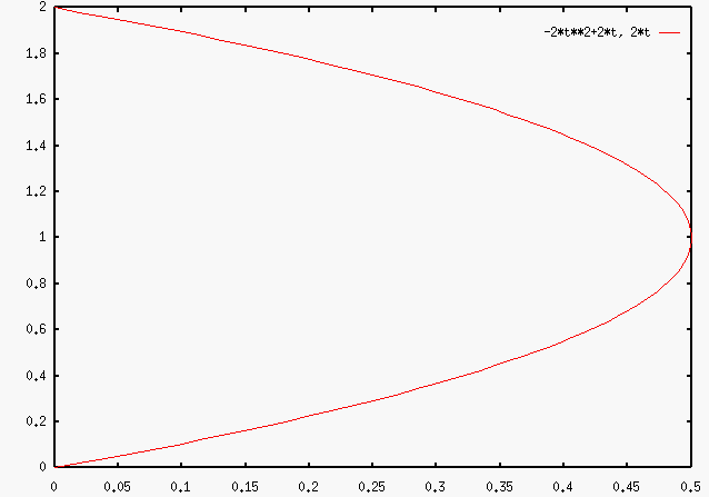
So, x = -2t2
+ 2t
y = 2t
(The curve is shown as above)
(c) First, we have to check the end
points of the two curves to determine C0
continuity.
Pa(t) = (3t2-1, t3-4t+1,
3t+2)
Pb(t) = (t2-1, 2t3-t2+8t+1,
t3-6t+2)
Pa(0) = (-1, 1, 2)
Pb(0) = (-1, 1, 2)
So, when t = 0, C0 continuous.
Pa(1) = (2, -2, 5)
Pb(1) = (0, 10, -3)
So,the beginning of two curves joint at the
same point when t = 0.
Now check for the first derivatives of both
curves at t = 0
P'a(t) = (6t, 3t2-4, 3)
P'b(t) = (2t, 6t2-2t+8,
3t2-6)
P'a(0) = (0, -4, 3)
P'b(0) = (0, 8, -6)
Therefore
-2P'a(0) = P'b(0)
Since their first derivatives are negatively
proportional at the same point, they do not
have the same direction.
So we can conclude that Pa(t)
and Pb(t) are only C0
continuous.
3(b)
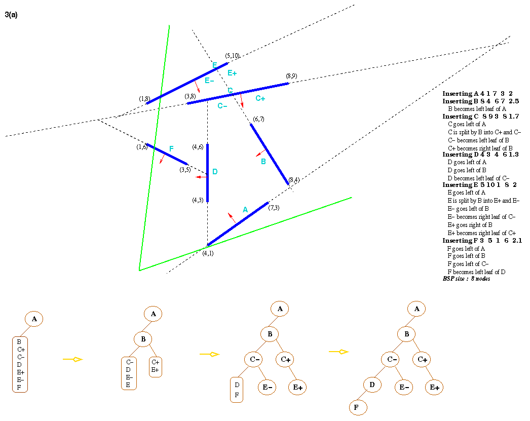
The program prints out the number of nodes in the completed
BSP tree. This can be more than
the number of polygons because some of them are split when they
are inserted into tree. The
insertion order of polygons can yield an optimal (e.g., minimal size)
BSP tree for test1.
The
best way to generate an optimal BSP tree is to minimize number of divided
partitioning
planes (i.e. avoid dividing a node into two separate ones.) In other
words, the smaller the
BSP tree size (must be greater or equal to number of partitioning planes),
the optimal
the BSP tree is.
The followings are two examples that yield an optimal BSP tree for test1.
i) MyTest1 Script File
A 4 1 7 3 2
C 8 9 3 8 1.7
E 1 8 5 10 2
B 8 4 6 7 2.5
D 4 6 4 3 1.3
F 1 6 3 5 2.1
hactar% bsp -d < MyTest1
Inserting A 4 1 7 3 2
Inserting C 8 9 3 8 1.7
C becomes left leaf of A
Inserting E 5 10 1 8 2
E goes left of A
E becomes right leaf of C
Inserting B 8 4 6 7 2.5
B goes left of A
B becomes left leaf of C
Inserting D 4 3 4 6 1.3
D goes left of A
D goes left of C
D becomes left leaf of B
Inserting F 3 5 1 6 2.1
F goes left of A
F goes left of C
F goes left of B
F becomes left leaf of D
BSP size: 6 nodes
ii) MyTest2 Script File
E 1 8 5 10 2
C 8 9 3 8 1.7
A 4 1 7 3 2
B 8 4 6 7 2.5
D 4 6 4 3 1.3
F 1 6 3 5 2.1
hactar% bsp -d < MyTest2
Inserting E 5 10 1 8 2
Inserting C 8 9 3 8 1.7
C becomes left leaf of E
Inserting A 4 1 7 3 2
A goes left of E
A becomes left leaf of C
Inserting B 8 4 6 7 2.5
B goes left of E
B goes left of C
B becomes left leaf of A
Inserting D 4 3 4 6 1.3
D goes left of E
D goes left of C
D goes left of A
D becomes left leaf of B
Inserting F 3 5 1 6 2.1
F goes left of E
F goes left of C
F goes left of A
F goes left of B
F becomes left leaf of D
BSP size: 6 nodes
Insertion order for MyTest1
: A -> C -> E -> B -> D -> F
Insertion order for MyTest2
: E -> C -> A -> B -> D -> F
Since the BSP tree
sizes for the above scripts, MyTest1 and MyTest2, are both
6 nodes, which
are equal to the number
of partitioning planes inserted, we can conclude that both scripts yield
optimal BSP trees.
Note that it is possible to generate other optimal BSP trees with different
insertion orders.
3(c) By inspection we know that test3
is the worst-order for the number of nodes in a BSP tree if
the
scene contains
n polygons, whereas test4 is the best-order for the number of nodes
in a BSP tree
in the same
condition.
The following diagram illustrates the insertion order of test3 and test4 :
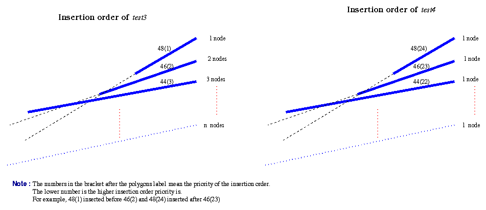
Assume the scene contains n polygons
Test4(Best-case)
The total
number of node, S = 1 + 1 + 1 + ...... + 1
S = n
Test3(Worst-case)
The total
number of node, S = 1 + 2 + 3 + .......... + n
S = 1 + 2 +
3 + 4
+ ..... + (n-1) + n
+ S = n + (n-1) + (n-2) +
(n-3) + ..... + 2 + 1
----------------------------------
2S = n (n+1)
S = n (n +1) / 2
Thus the worst-case order for the
number of nodes in a BSP tree if the scene contains n polygons
is n (n+1) / 2
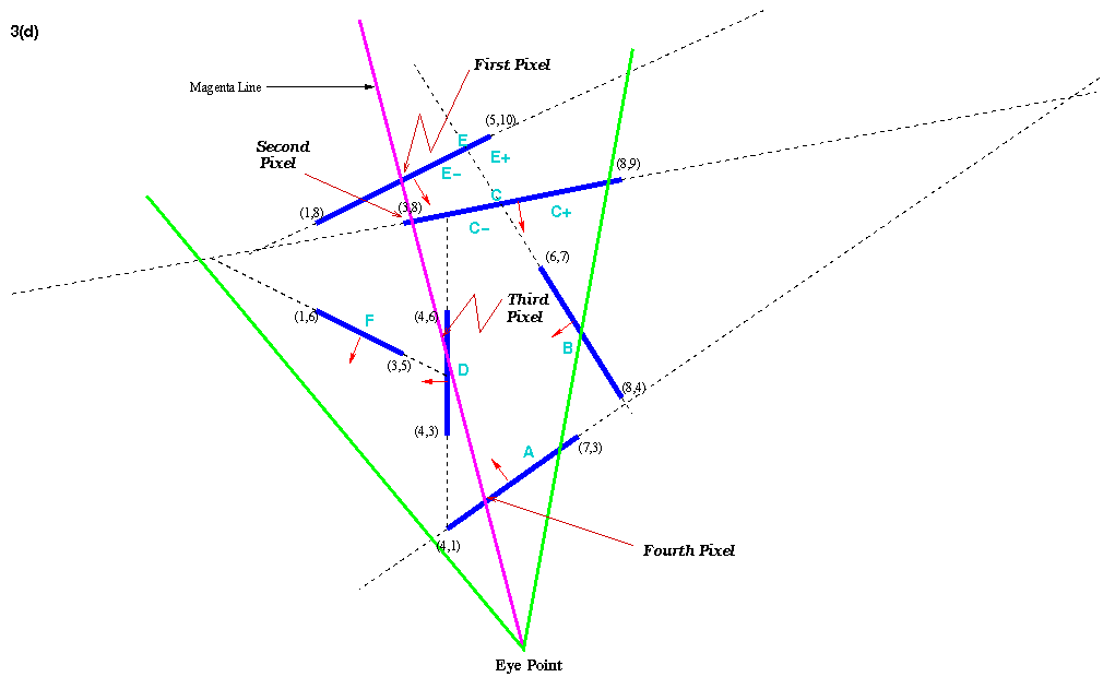
By inspection from the diagram above, we know
that the maximum depth complexity that the scene
test1 can exhibit is 4.
This can be seen at the magenta line
shown as above. It is possible to have
different pixels to get the maximum depth
complexity that the scene test1 can exhibit but the
maximum depth complexity for this particular
scene is 4.